Skyline timeseries异常判定算法
Skyline内部提供了9个预定义的算法,这些算法要解决这样一个问题:
input:一个timeseries
output:是否异常
3-sigma
一个很直接的异常判定思路是,拿最新3个datapoint的平均值(tail_avg方法)和整个序列比较,看是否偏离总体平均水平太多。怎样算“太多”呢,因为standard deviation表示集合中元素到mean的平均偏移距离,因此最简单就是和它进行比较。这里涉及到3-sigma理论:
In statistics, the 68–95–99.7 rule, also known as the three-sigma rule or empirical rule, states that nearly all values lie within 3 standard deviations of the mean in a normal distribution.
About 68.27% of the values lie within 1 standard deviation of the mean. Similarly, about 95.45% of the values lie within 2 standard deviations of the mean. Nearly all (99.73%) of the values lie within 3 standard deviations of the mean.
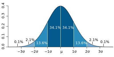
简单来说就是:在normal distribution(正态分布)中,99.73%的数据都在偏离mean 3个σ (standard deviation 标准差) 的范围内。如果某些datapoint到mean的距离超过这个范围,则认为是异常的。Skyline初始内置的7个算法几乎都是基于该理论的:
stddev_from_average
def stddev_from_average(timeseries):
    """
    A timeseries is anomalous if the absolute value of the average of the latest
    three datapoint minus the moving average is greater than one standard
    deviation of the average. This does not exponentially weight the MA and so
    is better for detecting anomalies with respect to the entire series.
    """
    series = pandas.Series([x[1] for x in timeseries])
    mean = series.mean()
    stdDev = series.std()
    t = tail_avg(timeseries)

    return abs(t - mean) > 3 * stdDev
该算法如下:
- 求timeseries的mean
- 求timeseries的standard deviation
- 求tail_avg到mean的距离,大于3倍的标准差则异常。
该算法的特点是可以有效屏蔽 “在一个点上突变到很大的异常值但在下一个点回落到正常水平” 的情况,即屏蔽单点毛刺:因为它使用的是末3个点的均值(有效缓和突变),和整个序列比较(均值可能被异常值拉大),导致判断正常。对于需要忽略 “毛刺” 数据的场景而言,该算法比后续的EWMA/mean_subtraction_cumulation等算法更适用(当然也可以改造这些算法,用tail_avg代替last datapoint)。
first_hour_average
def first_hour_average(timeseries):
    """
    Calcuate the simple average over one hour, FULL_DURATION seconds ago.
    A timeseries is anomalous if the average of the last three datapoints
    are outside of three standard deviations of this value.
    """
    last_hour_threshold = time() - (FULL_DURATION - 3600)
    series = pandas.Series([x[1] for x in timeseries if x[0] < last_hour_threshold])
    mean = (series).mean()
    stdDev = (series).std()
    t = tail_avg(timeseries)

    return abs(t - mean) > 3 * stdDev
和上述算法几乎一致,但是不同的是,比对的对象是 最近FULL_DURATION时间段内开始的1小时内 的数据,求出这段datapoint的mean和standard deviation后再用tail_avg进行比较。当FULL_DURATION小于1小时(86400)时,该算法和上一个算法一致。对于那些在一段较长时间内匀速递增/减的metrics,该算法可能会误报。
stddev_from_moving_average
def stddev_from_moving_average(timeseries):
    """
    A timeseries is anomalous if the absolute value of the average of the latest
    three datapoint minus the moving average is greater than one standard
    deviation of the moving average. This is better for finding anomalies with
    respect to the short term trends.
    """
    series = pandas.Series([x[1] for x in timeseries])
    expAverage = pandas.stats.moments.ewma(series, com=50)
    stdDev = pandas.stats.moments.ewmstd(series, com=50)

    return abs(series.iget(-1) - expAverage.iget(-1)) > 3 * stdDev.iget(-1)
该算法先求出最后一个datapoint处的EWMA(Exponentially-weighted moving average)mean/std deviation,然后用最后 3 个datapoint的平均值与之比对,看是否满足3-sigma理论。
关于 Moving Average
给定一个timeseries和subset长度(比如N天),则datapoint i 的N天 moving average = i之前N天(包括i)的平均值。不停地移动这个长度为N的“窗口”并计算平均值,就得到了一条moving average曲线。
Moving average常用来消除数据短期内的噪音,显示长期趋势;或者根据已有数据预测未来数据。
Simple Moving Average
这是最简单的moving average,为“窗口”内datapoints的算数平均值(每个datapoint的weight一样):
SMA(i) = [p(i) + p(i-1) + … + p(i-n+1) ]/ n
当计算i+1处的SMA时,一个新的值加入,“窗口”左端的值丢弃,因此可得到递推式:
SMA(i) = SMA(i-1) + p(i)/n – p(i-n+1)/n
实现起来也很容易,只要记录上次SMA和将要丢弃的datapoint即可(最开始的几个是没有SMA的)。Pandas中可用 pandas.stats.moments.rolling_mean 计算SMA。
SMA由于过去的数据和现在的数据权重是一样的,因此它相对真实数据的走向存在延迟,不太适合预测,更适合观察长期趋势。
Exponential moving average
也称 Exponential-weighted moving average,它和SMA主要有两处不同:
计算SMA仅“窗口”内的n个datapoint参与计算,而EWMA则是之前所有point;
EWMA计算average时每个datapoint的权重是不一样的,最近的datapoint拥有越高的权重,随时间呈指数递减。
EWMA的递推公式是:
EWMA(1) = p(1)  // 有时也会取前若干值的平均值。α越小时EWMA(1)的取值越重要。
EWMA(i) = α * p(i) + (1-α) * EWMA(i – 1) // α是一个0-1间的小数,称为smoothing factor.
可以看到比SMA更容易实现,只要维护上次EWMA即可。
EWMA 的本质其实是,越老的数据在预测时占的比例越低。扩展以上公式可以看到,从i往前的datapoint,权重依次为α, α(1-α), α(1-α)^2….., α(1-α)^n,呈指数递减,权重的和的极限等于1。
smoothing factor决定了EWMA的 时效性 和 稳定性。α越大时效性越好,越能反映出最近数据状态;α越小越平滑,越能吸收瞬时波动,反映出长期趋势。
EWMA由于其时效性被广泛应用在“根据已有时间序列预测未来数据”的场景中,(在计算机领域)比较典型的应用是在TCP中估计RTT,即从已有的RTT数据计算未来RTT,以确定超时时间。
虽然EWMA中参与计算的是全部datapoint,但它也有类似SMA “N天EWMA”的概念,此时α由N决定:α = 2/(N+1),关于这个公式的由来参见这里。
回到Skyline,这里并不是用EWMA来预测未来datapoint,而是类似之前的算法求出整体序列的mean和stdDev,只不过计算时加入了时间的权重(EWMA),越近的数据对结果影响越大,即判断的参照物是最近某段时间而非全序列; 再用last datapoint与之比较。因此它的优势在于:
- 可以检测到一个异常较短时间后发生的另一个(不太高的突变型)异常,其他算法很有可能会忽略,因为第一个异常把整体的平均水平和标准差都拉高了
- 比其他算法更快对异常作出反应,因为它更多的是参考突变之前的点(低水平),而非总体水平(有可能被某个异常或者出现较多次的较高的统计数据拉高)
而劣势则是
- 对渐进型而非突发型的异常检测能力较弱
- 异常持续一段时间后可能被判定为正常
mean_subtraction_cumulation
def mean_subtraction_cumulation(timeseries):
    """
    A timeseries is anomalous if the value of the next datapoint in the
    series is farther than a standard deviation out in cumulative terms
    after subtracting the mean from each data point.
    """

    series = pandas.Series([x[1] if x[1] else 0 for x in timeseries])
    series = series - series[0:len(series) - 1].mean()
    stdDev = series[0:len(series) - 1].std()
    expAverage = pandas.stats.moments.ewma(series, com=15)

    return abs(series.iget(-1)) > 3 * stdDev
算法如下:
- 排除全序列(暂称为all)最后一个值(last datapoint),求剩余序列(暂称为rest,0..length-2)的mean;
- rest序列中每个元素减去rest的mean,再求standard deviation;
- 求last datapoint到rest mean的距离,即 abs(last datapoint – rest mean);
- 判断上述距离是否超过rest序列std. dev.的3倍。
简单地说,就是用最后一个datapoint和剩余序列比较,比较的过程依然遵循3-sigma。这个算法有2个地方很可疑:
- 求剩余序列的std. dev.时先减去mean再求,这一步是多余的,对结果没影响;
- 虽然用tail_avg已经很不科学了,这个算法更进一步,只判断最后一个datapoint是否异常,这要求在两次analysis间隔中最多只有一个datapoint被加入,否则就会丢失数据。关于这个问题的讨论,见这篇文章最末。
和stddev_from_average相比,该算法对于 “毛刺” 判断为异常的概率远大于后者。
least_squares
def least_squares(timeseries):
    """
    A timeseries is anomalous if the average of the last three datapoints
    on a projected least squares model is greater than three sigma.
    """

    x = np.array([t[0] for t in timeseries])
    y = np.array([t[1] for t in timeseries])
    A = np.vstack([x, np.ones(len(x))]).T
    results = np.linalg.lstsq(A, y)
    residual = results[1]
    m, c = np.linalg.lstsq(A, y)[0]
    errors = []
    for i, value in enumerate(y):
        projected = m * x[i] + c
        error = value - projected
        errors.append(error)

    if len(errors) < 3:
        return False

    std_dev = scipy.std(errors)
    t = (errors[-1] + errors[-2] + errors[-3]) / 3

return abs(t) > std_dev * 3 and round(std_dev) != 0 and round(t) != 0- 用最小二乘法得到一条拟合现有datapoint value的直线;
- 用实际value和拟合value的差值组成一个新的序列error;
- 求该序列的stdDev,判断序列error的tail_avg是否>3倍的stdDev
因为最小二乘法的关系,该算法对直线形的metrics比较适用。该算法也有一个问题,在最后判定的时候,不是用tail_avg到error序列的mean的距离,而是直接使用tail_avg的值,这无形中缩小了异常判定范围,也不符合3-sigma。
小结
可以看到上述算法都是类似的思路:用最近的若干datapoint做样本,和一个总体序列进行比对,不同的只是比对的对象:
stddev_from_average
tail_avg ——— 整个序列first_hour_average
tail_avg ———- FULL_DURATION开始的一个小时stddev_from_moving_average
last datapoint ———– 整个序列的EW mean和EW std devmean_subtraction_cumulation
last datapoint ——— 剩余序列least_squares
last datapoint ——– 真实数据和拟合直线间的差值序列
grubbs
def grubbs(timeseries):
    """
    A timeseries is anomalous if the Z score is greater than the Grubb's score.
    """

    series = scipy.array([x[1] for x in timeseries])
    stdDev = scipy.std(series)
    mean = np.mean(series)
    tail_average = tail_avg(timeseries)
    z_score = (tail_average - mean) / stdDev
    len_series = len(series)
    threshold = scipy.stats.t.isf(.05 / (2 * len_series) , len_series - 2)
    threshold_squared = threshold * threshold
    grubbs_score = ((len_series - 1) / np.sqrt(len_series)) * np.sqrt(threshold_squared / (len_series - 2 + threshold_squared))

    return z_score > grubbs_score
Grubbs测试是一种从样本中找出outlier的方法,所谓outlier,是指样本中偏离平均值过远的数据,他们有可能是极端情况下的正常数据,也有可能是测量过程中的错误数据。使用Grubbs测试需要总体是正态分布的。
Grubbs测试步骤如下:
- 样本从小到大排序;
- 求样本的mean和std.dev.;
- 计算min/max与mean的差距,更大的那个为可疑值;
- 求可疑值的z-score (standard score),如果大于Grubbs临界值,那么就是outlier;
- Grubbs临界值可以查表得到,它由两个值决定:检出水平α(越严格越小),样本数量n
- 排除outlier,对剩余序列循环做 1-5 步骤。
由于这里需要的是异常判定,只需要判断tail_avg是否outlier即可。代码中还有求Grubbs临界值的过程,看不懂。
Z-score (standard score)
标准分,一个个体到集合mean的偏离,以标准差为单位,表达个体距mean相对“平均偏离水平(std dev表达)”的偏离程度,常用来比对来自不同集合的数据。
histogram_bins
def histogram_bins(timeseries):
    """
    A timeseries is anomalous if the average of the last three datapoints falls
    into a histogram bin with less than 20 other datapoints (you'll need to tweak
    that number depending on your data)

    Returns: the size of the bin which contains the tail_avg. Smaller bin size
    means more anomalous.
    """

    series = scipy.array([x[1] for x in timeseries])
    t = tail_avg(timeseries)
    h = np.histogram(series, bins=15)
    bins = h[1]
    for index, bin_size in enumerate(h[0]):
        if bin_size <= 20:
            # Is it in the first bin?
            if index == 0:
                if t <= bins[0]:
                    return True
            # Is it in the current bin?
            elif t >= bins[index] and t < bins[index + 1]:
                    return True

    return False
该算法和以上都不同,它首先将timeseries划分成15个宽度相等的直方,然后判断tail_avg所在直方内的元素是否<=20,如果是,则异常。
直方的个数和元素个数判定需要根据自己的metrics调整,不然在数据量小的时候很容易就异常了。
ks_test
def ks_test(timeseries):
    """
    A timeseries is anomalous if 2 sample Kolmogorov-Smirnov test indicates
    that data distribution for last 10 minutes is different from last hour.
    It produces false positives on non-stationary series so Augmented
    Dickey-Fuller test applied to check for stationarity.
    """

    hour_ago = time() - 3600
    ten_minutes_ago = time() - 600
    reference = scipy.array([x[1] for x in timeseries if x[0] >= hour_ago and x[0] < ten_minutes_ago])
    probe = scipy.array([x[1] for x in timeseries if x[0] >= ten_minutes_ago])

    if reference.size < 20 or probe.size < 20:
        return False

    ks_d,ks_p_value = scipy.stats.ks_2samp(reference, probe)

    if ks_p_value < 0.05 and ks_d > 0.5:
        adf = sm.tsa.stattools.adfuller(reference, 10)
        if  adf[1] < 0.05:
            return True

    return False
这个算法比较高深,它将timeseries分成两段:最近10min(probe),1 hour前 -> 10 min前这50分钟内(reference),两个样本通过Kolmogorov-Smirnov测试后判断差异是否较大。如果相差较大,则对refercence这段样本进行 Augmented Dickey-Fuller 检验(ADF检验),查看其平稳性,如果是平稳的,说明存在从平稳状态(50分钟)到另一个差异较大状态(10分钟)的突变,序列认为是异常的。
关于这两个检验过于学术了,以上只是我粗浅的理解。
Kolmogorov-Smirnov test
KS-test有两个典型应用:
判断某个样本是否满足某个已知的理论分布,如正态/指数/均匀/泊松分布;
判断两个样本背后的总体是否可能有相同的分布,or 两个样本间是否可能来自同一总体, or 两个样本是否有显著差异。
检验返回两个值:D,p-value,不太明白他们的具体含义,Skyline里当 p-value < 0.05 && D > 0.5 时,认为差异显著。Augmented Dickey-Fuller test (ADF test)
用于检测时间序列的平稳性,当返回的p-value小于给定的显著性水平时,序列认为是平稳的,Skyline取的临界值是0.05。
median_absolute_deviation
def median_absolute_deviation(timeseries):
    """
    A timeseries is anomalous if the deviation of its latest datapoint with
    respect to the median is X times larger than the median of deviations.
    """

    series = pandas.Series([x[1] for x in timeseries])
    median = series.median()
    demedianed = np.abs(series - median)
    median_deviation = demedianed.median()

    # The test statistic is infinite when the median is zero,
    # so it becomes super sensitive. We play it safe and skip when this happens.
    if median_deviation == 0:
        return False

    test_statistic = demedianed.iget(-1) / median_deviation

    # Completely arbitary...triggers if the median deviation is
    # 6 times bigger than the median
    if test_statistic > 6:
        return True
该算法不是基于mean/ standard deviation的,而是基于median / median of deviations (MAD)。
Median
大部分情况下我们用mean来表达一个集合的平均水平(average),但是在某些情况下存在少数极大或极小的outlier,拉高或拉低了(skew)整体的mean,造成估计的不准确。此时可以用median(中位数)代替mean描述平均水平。Median的求法很简单,集合排序中间位置即是,如果集合总数为偶数,则取中间二者的平均值。
Median of deviation(MAD)
同mean一样,对于median我们也需要类似standard deviation这样的指标来表达数据的紧凑/分散程度,即偏离average的平均距离,这就是MAD。MAD顾名思义,是deviation的median,而此时的deviation = abs( 个体 – median ),避免了少量outlier对结果的影响,更robust。
现在算法很好理解了:求出序列的MAD,看最后datapoint与MAD的距离是否 > 6个MAD。同样的,这里用最后一个datapoint判定,依然存在之前提到的问题;其次,6 是个“magic number”,需要根据自己metrics数据特点调整。
该算法的优势在于对异常更加敏感:假设metric突然变很高并保持一段时间,基于标准差的算法可能在异常出现较短时间后即判断为正常,因为少量outlier对标准差的计算是有影响的;而计算MAD时,若异常datapoint较少会直接忽略,因此感知异常的时间会更长。
但正如Median的局限性,该算法对于由多个cluster组成的数据集,即数据分布在几个差距较大的区间内,效果很差,很容易误判。比如下图:
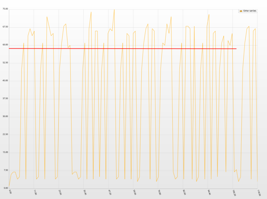
该曲线在两个区间内来回震荡,此时median为58,如红线所示。MAD计算则为9,很明显均不能准确描述数据集,最后节点的deviation=55,此时误判了。
参考资料
- 各种Wiki
- 各种API文档
- 前辈的总结:【Etsy 的 Kale 系统】skyline 的过滤算法
- Moving Averages: What Are They?
- Kolmogorov-Smirnov检验
- Grubbs检验法
- Median absolute deviation
- 《Head first statistics》